🚨 please pull a fresh copy of the codebase before starting this homework! 🗣️ you are highly encouraged to collaborate on homework provided you follow the spirit of the 50 ft rule 👥 additionally, for this lab you may optionally choose to work with a partner 📚 this writeup is long
goals. - get a first taste of physics-based animation - get a first taste of skeletal animation
a. pendulum Consider a 2D pendulum with length $L$ and mass $m = 1.0 \text{kg}$ concentrated at the bottom. Recall gravitational acceleration to be $g = -9.81 \text{m}/{\text{s}}^2$.
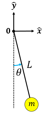 Notate the mass's angular position $\theta$, measured counter-clockwise from the negative $y$-axis.
It follow that the mass's spatial position is $\mathbf{p} = L\begin{bmatrix}\sin(\theta)\\ -\cos(\theta)\end{bmatrix}$
Notate the mass's angular position $\theta$, measured counter-clockwise from the negative $y$-axis.
It follow that the mass's spatial position is $\mathbf{p} = L\begin{bmatrix}\sin(\theta)\\ -\cos(\theta)\end{bmatrix}$
Call the mass's angular velocity $\omega = \dot\theta$ Call the mass's angular acceleration $\alpha = \ddot\theta$ Note that in "dot notation," the number of dots denotes the number of time derivatives. E.g., $\dot\theta = \frac{d\theta}{dt}$ and $\ddot\theta = \frac{d^2\theta}{dt^2}$. ✅ Note that $\dot\omega = \alpha$
The dynamics of a rotating rigid body are governed by (the torque form of) Newton's second law $$\tau = I\alpha,$$where $\tau$ is the torque about the axis of rotation, $I$ is the moment of inertia, and $\alpha$ is the angular acceleration. For our particular problem, the gravitational force on the pendulum's mass is $mg$, and the length of the perpendicular lever arm is $L\sin\theta$. Therefore, the torque about the axis of rotation is $\tau=mgL\sin\theta$. Additionally, recall (via Google or ChatGPT) that the moment of inertia of a point mass at distance $L$ from the axis of rotation is $I = mL^2$. Substituting these facts into Newton's second law yields $$mgL\sin\theta=mL^2\alpha$$This implies$${\alpha = \frac{g}{L}\sin\theta}$$✅ Note that $\alpha$ does not depend on $m$. What does this *mean*?
Call the state of the system$$\xi = \begin{bmatrix}\theta\\ \omega\end{bmatrix}$$ In order to simulate, we need to discretize our physics in time. The very useful notation $\xi_k$ means "$\xi$ at time $t_k$." Call $h = 0.0167 \text{s}$ the timestep length. If $\xi_{k}$ is the state of the system at time $t_k$, then $\xi_{k+1}$ will be the state of the system at time $t_{k+1} = t_k + h$. ✅ Note that $h$ is one sixtieth of a second. Since cow runs at 60fps, this makes our simulation real-time.
We can calculate the time derivative of a vector one component at a time, i.e., $$\dot\xi_k = \begin{bmatrix}\dot\theta_{k}\\\dot\omega_{k}\end{bmatrix} = \begin{bmatrix}\omega_{k}\\\alpha_{k}\end{bmatrix}$$
Implement the following integration methods. Explicit (Forward) Euler is $\xi_{k + 1} = \xi_{k} + h \dot\xi_{k}$ It should gain energy over time. Semi-Implicit (Symplectic) Euler, for our problem, ends up being $\begin{bmatrix}\theta_{k+1}\\\omega_{k+1}\end{bmatrix} = \begin{bmatrix}\theta_{k}\\\omega_{k}\end{bmatrix} + h\begin{bmatrix}\omega_{k + 1}\\\alpha_{k}\end{bmatrix} $ It should preserve energy over time. Note: If this equation feels like it kind of came out of nowhere, you may be interested in the supplemental reading linked at the end of the pendulum problem. Implicit (Backward) Euler is $\xi_{k + 1} = \xi_{k} + h \dot\xi_{k + 1}$ It should lose energy over time.
Note that $\xi_{k + 1}$ shows up on both sides of the Implicit Euler update rule. For our problem, this will make the update rule impossible to solve analytically for $\xi_{k + 1}$. We can instead solve for $\xi_{k + 1}$ numerically. A numerical technique called fixed-point iteration works well for our problem. Here is a simple (runnable) example of fixed-point iteration to solve the equation $x = cos(x)$. It initializes $x \leftarrow 0$.
real x = 0.0;
real prevEstimate;
do {
    prevEstimate = x;
    x = cos(x);
} while (!ARE_EQUAL(prevEstimate, x));
printf("%x = cos(x) at lf\n", x);
For our problem, note that the time derivative of the next state is a function of the next state $\dot\xi_{k+1} = \mathbf{f}(\xi_{k + 1}).$
(Hint / Concept Check) Specifically,
$$\mathbf{f}(\xi_{k + 1}) = \begin{bmatrix}\omega_{k + 1}\\\alpha_{k + 1}\end{bmatrix} = \begin{bmatrix}\omega_{k + 1}\\\frac{g}{L}\sin\theta_{k+1}\end{bmatrix}$$(Spoilers) Here is my fixed-point iteration for our problem:
vec2 curr = ...;  // $\xi_k$
vec2 next = curr; // $\xi_{k + 1}$
while (true) {
    // $\xi_{k + 1}^{est} = \xi_k + h * f(\xi_{k + 1}^{est})
    vec2 tmp = curr + h * V2(next[1], get_alpha(next[0]));
    if (IS_ZERO(squaredNorm(next - tmp))) { break; }
    next = tmp;
}
(Optional) Supplementary Reading. 🐧 Implement explicit euler integration for a double pendulum (you will want to take very small timesteps). You can also try to implement semi-implicit euler and implicit euler if you would like.
b. linear blend skinning
Note: We won't actually write coordiante systems as homogeneous matrices to solve the homework problem. However, the following derivation will give you a concise, general understanding of linear blend skinning. I recommend drawing pictures as you read.
Here is the general purpose 3D derivation. Consider a skeleton made of bones. Call $\mathbf{B}_j$ the coordinate system attached to the $j$-th bone in the skeleton, in world coordinates. Note that for a 3D mesh, $\mathbf{B}_j$ will be a 4x4 matrix. Consider a skin made of nodes. Call $\mathbf{s}_i$ the position of the i-th node in the skin, in world coordinates. Consider the skeleton and skin in a choice of binding pose (e.g., "T-pose", with the character's arms stuck straight out). In the binding pose, we say that the $j$-th bone's coordinate system is $\mathbf{B}_j^{\text{bind}}$ and the $i$-th node's position is $\mathbf{s}_i^{\text{bind}}$, all in world coordinates. Call ${}_j{\mathbf{s}_i} = \left(\mathbf{B}_j^{\text{bind}}\right)^{-1} \mathbf{s}_i^{\text{bind}}$ the $i$-th node's position in the $j$-th bone's coordinate system. Now we move the skeleton around. We can calculate $\mathbf{t}_{ij} = \mathbf{B}_j\ {}_j{\mathbf{s}_i}$ the position of the $i$-th node if we had bolted it to the $j$-th bone when everything was in the bind pose. Note that $\mathbf{t}_{ij}$ is in world coordinates. In practice, rather than attach the node to a single bone, we blend the result of attaching it to each of the bones by means of a weighted average (a special kind of linear combination where the sum of the weights/coefficients is 1). Call $W_{ij}$ the weight of the $j$-th bone on the $i$-th node, where we are careful to ensure $\sum_j W_{ij} = 1.$ Note: the weights are computed (initalized) only once, typically with respect to the bind pose. I.e., the weights do not change over time. They are constants. This way of calculating the position of the skin is called linear blend skinning:$$\boxed{\mathbf{s_i} = \sum_{j} W_{ij} \mathbf{t}_{ij}}$$
For our simple 2D setup, the general-purpose matrix solution might be overkill. Instead, we'll start from the idea that each (2D) bone has a 2D position $\mathbf{b}_j$ and a 1D angle $\theta_j$, both in world coordinates. I recommend trying to figure how this approach works on paper; there are spoilers below if you get stuck or would like to see my particular solution.
(Hint / Spoilers) How to compute $\mathbf{b}_j$
We place the left side of the zeroth bone at the origin, i.e., $\mathbf{b}_j = \mathbf{0}$. Then $\mathbf{b}_{j + 1} = \mathbf{b}_j + L_j \hat{\mathbf{e}}_\theta,$ where $\hat{\mathbf{e}}_\theta=\begin{bmatrix}\cos\theta\\\sin\theta\end{bmatrix}.$(Hint / Spoilers) How to compute ${}_j{\mathbf{s}_i}$
We have ${}_j{\mathbf{s}_i} = \mathbf{s}_i^{\text{bind}} - \mathbf{b}_j^{\text{bind}}$.(Hint / Spoilers) How to compute $\mathbf{t}_{ij}$
Finally $\mathbf{t}_{ij} = \mathbf{b}_j + \mathbf{R}_{\theta_j}\ {}_j{\mathbf{s}_i}$.These snail functions may be convenient:
vec2 rotated(vec2 a, real theta);
returns the result of rotating a vector (or point) a counter-clockwise by theta, i.e., $\mathbf{R}_\theta\ \mathbf{a} = \begin{bmatrix}\cos\theta & -\sin\theta \\ \sin\theta & \cos\theta\end{bmatrix}\begin{bmatrix}a_x\\a_y\end{bmatrix}$
vec2 e_theta(real theta);
returns a unit vector with angle theta, i.e., $\hat{\mathbf{e}}_\theta = \begin{bmatrix}\cos\theta\\\sin\theta\end{bmatrix}$.
✅ e_theta(theta) returns the same thing as rotated(V2(1.0, 0.0), theta).
Additionally, you are given a useful function
real point_segment_distance(vec2 p, vec2 a, vec2 b);.
Implement forward kinematics (calculate $\mathbf{b}_j$ for $j=0,1,...,\text{NUM_BONES}$) in
update_skeleton(...).
Once you are done, you should be able to move the skeleton around by pressing 'p' on the keyboard or by playing with the sliders.
(Spoiler)
    b[0] = {};
    for (int j = 0; j < NUM_BONES; ++j ) {
        b[j + 1] = b[j] + L[j] * e_theta(theta[j]);
}update_skin(...).
Once you are done, you should see the skin around the skeleton. Note: the skin will NOT behave as you might expect when you move the skeleton. This is A-OK. I have implemented incorrect but educational approaches to initializing the weights $W_{ij}$. Take a look in the code for initialize_weights(...) and see if you can figure out what is going on for mode 0 (only-zeroth) and mode 1 (all-equal). Does the skin behave as you would expect now? Cool! Let's implement some proper skinning modes.
(Spoiler)
    for (int i = 0; i < NUM_NODES; ++i) {
        s[i] = {};
        for (int j = 0; j < NUM_BONES; ++j) {
            s[i] += weights[i][j] * (b[j] + rotated(s_bind[i] - b_bind[j], theta[j]));
        }
}initialize_weights(...).
In order to test rigid weights, switch the mode to rigid either by moving the slider or pressing 'k' twice on the keyboard. A correct implementation of rigid weights should look like a rigid robot (very "angular"). There will be some "artifacts" where triangles overlap each other.
Implement smooth weights in initialize_weights(...).
In order to test smooth weights, switch the mode to smooth either by moving the slider of pressing 'k' three times on the keyboard (if you're in a rush, you could instead press 'j' once). A correct implementation of smooth weights should look like a snake ("smooth"). All artifacts should be gone. :)
(Optional) Note that in practice, we would implement skinning in a vertex shader. 🦴 Make a new app that does skinning in 3D. You may use the matrix version if you like. You may do your skinning in a vertex shader if you like.
c. final project proposal In the glow comment for this hw, please answer final project questions 0-4 from the course homepage.